Final Video:
In our final project for this course, we chose to extend pathtracer, the class’s raytracer project, enabling real-time raytracing of 3D reconstructed scenes. Our project was split into two distinct components, one part responsible for optimizing raytracing for real-time performance, and one part responsible for entering 3D reconstructed scenes into our raytrace pipeline. We achieved the first part of our project through a combination of diffuse texture baking techniques to lower the raytracing load per frame, bidirectional raytracing, and replacing monte carlo integration with real integration. We achieved the second part of our project by diving into the collada parser and adding bits and pieces throughout the system in order to enable large-scale meshes with tens of thousands of individually colored triangles.
Part 1: Optimizations to achieve real-time performance
Texture Baking
The first technique that accounted for a giant leap in performance in our raytracing engine is texture baking. Texture baking takes advantage of surfaces with diffuse uniform BSDFs in order to precompute the effect of raytracing and global illumination on such surfaces. In this manner, we managed to greatly reduce the work performed by the raytracer during runtime. Instead of needing to perform a call to sample_f during each ray intersection with a diffuse surface, we can instead sample the associated texture to find the precomputed radiance at any point. Texture baking is commonly used in the video game industry to provide realistic scenes without the ability to ray trace in real-time (although Nvidia’s new RTX architecture promises the real thing).
This was implemented by performing a baking phase prior to runtime. While raytracing the scene, any intersection with a surface with a diffuse BSDF would perform a mapping from the intersection point to a unique position in a 2D vector, which would then be saved to an 8-bit 3-channel color image which would then be reloaded later for use during runtime.
Due to the implementation requiring one image per object in the scene, this made it infeasible to bake reconstructed scenes with over 100k+ individual triangles. This limited our ability to speed up the performance of ray tracing during real scenes, as without texture baking we needed to resort to other optimizations to improve performance.
Another major benefit that came along with texture baking was the ability to rasterize diffuse surfaces in the camera frame rather than ray trace at those pixels. Rasterizing is different from ray tracing in that it simply fills the frame buffer at the projected pixel in the image plane and is much faster than ray tracing at the cost of global illumination. However, with precalculated textures for diffuse surfaces already accounting for the effects of lighting in the scene, we could very easily emulate global illumination while rasterizing. This even further reduced the required workload of the pathtracer during runtime. Not only did the rays no longer have to path trace once intersecting with a diffuse surface, only rays pointing at non-diffuse surfaces from the camera’s perspective at the very onset would need to be ray traced in the first place. Rasterizing allowed the use of standard GPU hardware acceleration, further decreasing load on the CPU.
Bidirectional Ray Tracing / Photon mapping
In order to achieve less noisy scenes at a lower cost, we implemented bidirectional ray tracing. Originally, in pathtracer, ray tracing was performed from every pixel on the image plane and shot outwards into the scene and gathered radiance from every object it intersected with. However, in bidirectional ray tracing, rays are also shot outwards from light sources in the scene (or, in this case, the environment map) and their intersections with objects in the scene are recording in the baked texture of the objects. This allows for higher convergence on caustics in the scene, as well as higher accuracy in terms of global illumination. Most importantly, this improvement comes at little cost to the ray tracer during runtime, as the effects of bidirectional ray tracing are all stored inside the baked textures, which can be accessed as before in constant time.
Miscellaneous Optimizations
In order for the ray tracer to reach realtime performance on the CPU, shortcuts needed to be made. First, the sample rate for the raytracer was set to 1. Even with most of the scene comprising of diffuse surfaces able to be rasterized, a higher sample rate would severely damage performance.
Second, all dynamic allocations were removed during runtime. The only malloc/new operations occur inside OpenGL calls, which is unavoidable.
Third, no light sampling was run by the ray tracer during runtime. This was powered by the texture baking process, removing the need to sample lights during runtime because the only raytraced BSDFs were delta materials, which by definition can’t use light sampling.
Fourth, two BVH intersections were calculating in parallel using SIMD (single instruction, multiple data) functions to decrease the calculation time even further.
Fifth, we used the OpenGL rasterization result to perform initial ray intersections. Non-baked objects are still rasterized and their primitive index is encoded into the rasterization color. Then, when the pixel is raytraced, the intersected primitive is looked up in a table using the encoded color. This saves a BVH traversal for every initial ray in the scene, which is significant.
Ditching Monte Carlo
One of the consequences of only sampling once per pixel is no longer being able to render materials with multiple possible bounce directions (i.e. glass, microfacets) properly. One of the properties of glass is that some proportion of light is reflected while the rest is refracted. During the basic path tracer implementation, this is accounted for by directing some p proportion of the samples to refract and (1-p) of the samples to reflect. With only one sample, this clearly no longer functions. Therefore, we abandon Monte Carlo integration for glass and instead perform analytic integration. This slows down performance but produces overall faster speeds when used in conjunction with only one sample per pixel. While other materials can bounce in multiple directions (microfacets), we only use this optimization for glass because there is a finite number of bounces needed to achieve an accurate result (2 vs »>2).
Part 2: Reconstructed Scenes
Obtaining Reconstructions of Real Scenes
In order to perform reconstructions of real scenes, we used OpenARK’s 3D reconstruction module. OpenARK is Berkeley’s open-source augmented reality SDK developed by Berkeley’s FHL Vive Center for Enhanced Reality under Professor Allen Yang. One of our team members (Adam) works on the 3D reconstruction team and already had the hardware and software capabilities to perform 3D reconstructions. The 3D reconstructed meshes were constructed using pose-estimated RGB and depth images to generate a TSDF (truncated signed distance field) and then Marching Cubes was used to generate the triangle mesh from the TSDF. The underlying mechanisms of the 3D reconstruction system are detailed in Open3D’s paper, http://vladlen.info/papers/scene-reconstruction-POI.pdf.
After generating a colored triangle mesh, the meshes were processed in the following order to make them compatible with the pathtracer system.
Removed non-connected components. This step was necessary as the mesh would be transferred from an unordered triangle list to a half-edge data structure, requiring the entire mesh to be one connected component. Simplify meshes. Using MeshLab’s quadric edge collapse decimation, we reduced the number of triangles in a scene as much as possible while maintaining as much detail as possible. This is necessary to approach anything close to realtime performance.
- Removed non-connected components. This step was necessary as the mesh would be transferred from an unordered triangle list to a half-edge data structure, requiring the entire mesh to be one connected component.
- Simplify meshes. Using MeshLab’s quadric edge collapse decimation, we reduced the number of triangles in a scene as much as possible while maintaining as much detail as possible. This is necessary to approach anything close to realtime performance.
- Removed non-manifold faces and vertices. This step was also necessary to ensure a well-formed half-edge data structure.
- Convert to a .dae file format. This simply required transferring the vertices, triangles, and vertex colors to a .dae structure. We used meshconvert.com to perform this process.
- Insert mesh into scene with manually placed lighting.
- Manually indicate which triangles would need a different BSDF from diffuse.
Post-Processing of Real Scene Reconstructions
After reconstructing a scene as described above, certain modifications to the scene required some degree of manual intervention. While the process of removing zero-area faces, non-manifold edges, etc was mostly automated, the initial reconstruction was manually passed through Blender. From here, desired faces (triangles corresponding to windows for example), were manually selected and marked for post-processing to set proper BSDFs.
The resulting DAE’s were processed through a python script converting tagged BSDF’s such that they were compatible with the Pathtracer.
Supplemental Scenes constructed with Blender
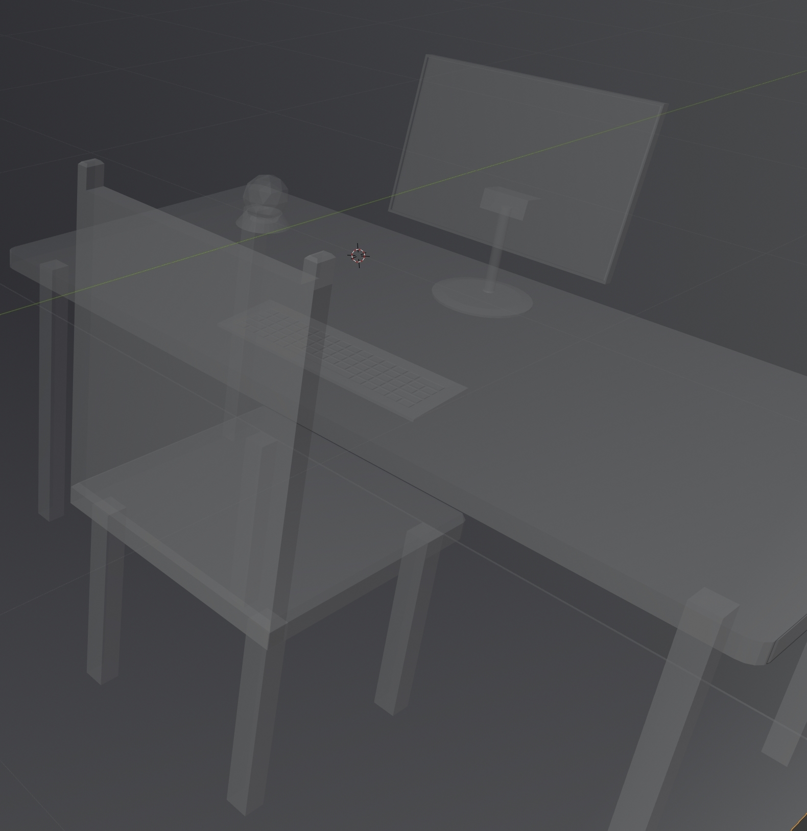
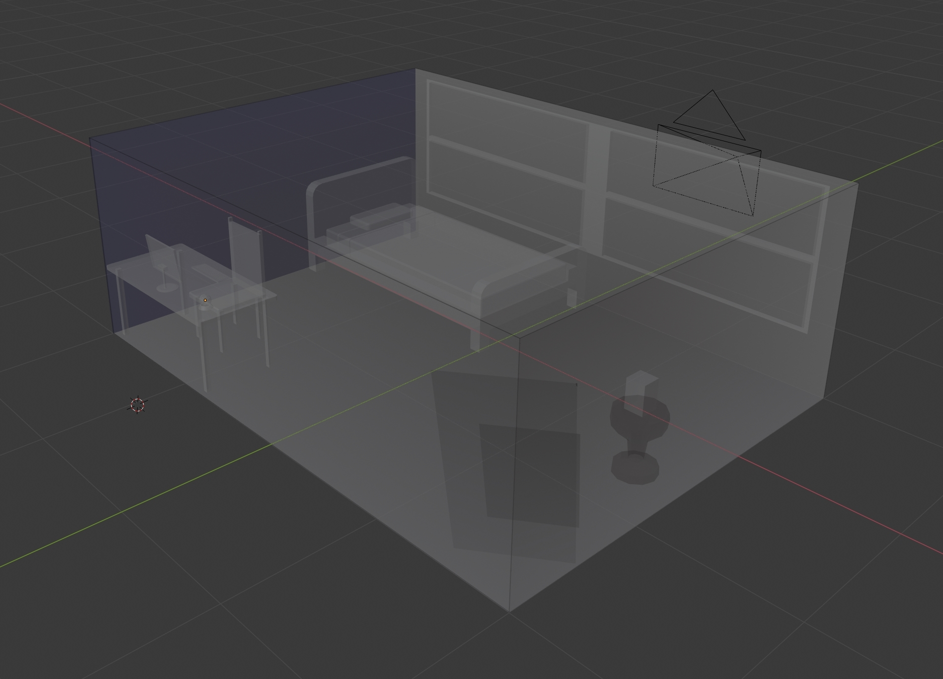
In order to effectively demonstrate the achievements of the real-time rendering engine, we constructed low-poly scenes in Blender, using multiple mirror and glass BSDF’s, along with standard diffuse BSDF’s to fully demonstrate the capabilities of the engine. In order to use Blender, some minor post-processing was necessary to generate DAE’s compatible with the Pathtracer. For our final demo results, we used these fabricated scenes as a substitute to the much larger, much more complex real scenes.
Miscellaneous Issues Encountered
Vertex Normals at Boundaries
During the course of adding custom meshes to pathtracer, we discovered that the computeNormals() function during the construction of the half-edge mesh data structure functioned improperly at the boundary vertices of meshes. The normals pointed in exactly the opposite direction as the normals of the vertices in the rest of the mesh. This resulted in a white outline around the backside of a mesh (normally all black) and a black outline around the frontside of a mesh (normally colored). We fixed this by implementing a new computeNormals() function without this bug.
Vertex Normals in the mesh.dae
We found another interesting issue stemming our use of meshconvert.com to generate the .dae file from our .ply file. The normals of the vertices were once again backwards from their proper orientation. The result was a mesh that displayed its colors on the wrong side of the mesh surface. We fixed this issue in a hacky fashion by simply adding a line normal = -normal inside computeNormals().
Results
We obtained several promising results from our optimizations with regards to real time raytracing of virtual scenes.
Texture baking was very successful. Compare the speedup gained when using baking to render scenes at a similar level of detail (~2 minutes of baking needed):
and with baking:
Next, rasterizing baked textures was also very successful and allowed us to skip raytracing for most of the pixels in a given scene (slowed down for effect, otherwise raytracing is near instantaneous). Because most of the scene is comprised of diffuse surfaces, true ray tracing is only needed during runtime for the glass and mirror spheres as well as the mirror along the back wall.
Using rasterization to perform intersections gave a noticeable 20% speedup, which you can see in this slowed down comparison (in addition to the intersections encoded as colors):
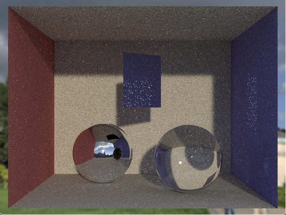
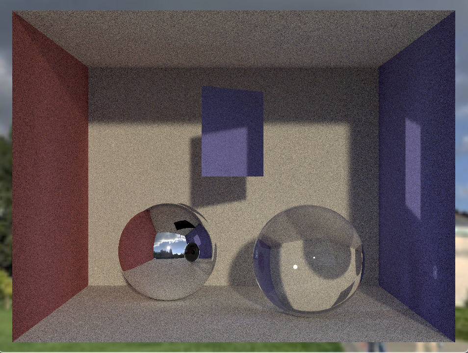
Bidirectional raytracing greatly improved the quality of our bakes for a given amount of time. This comparison illustrates the caustics generated through bidirectional ray tracing (right) versus through unidirectional ray tracing (left). Because each light source is individually ray traced through each refractive object in the scene, the resulting caustics are much more defined at lower bake times.
|
|
|
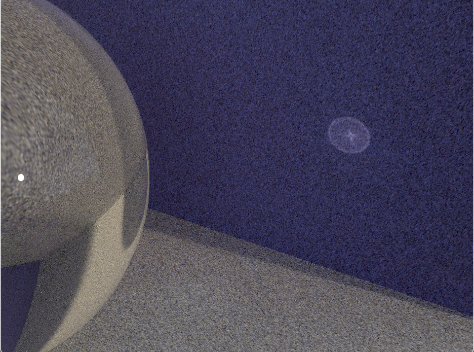
|
This comparison illustrates the effect of analytic integration (right) versus Monte Carlo integration (left), given we are using only one sample per ray. The Monto Carlo integration is doomed to failure as glass requires multiple rays to properly be sampled, as rays have different behaviors with varying probability (described by Fresnel equations). Analytic integration is slower, but worth it for the realistic effects.
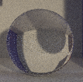
|
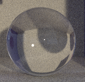
|
We found it was very hard to incorporate both texture baking and reconstructed scenes while keeping the realtime aspect. Because of this, we have to relax one of the constraints. A scene with only rasterization (no mirrors or glass in view) could run at 30 fps for a reasonable amount of triangles (e.g. a few thousand), but the reconstructions consisted of hundreds of thousands of triangles, or tens of thousands after significant simplification. Drawing hundreds of thousands of triangles each with a unique texture in OpenGL isn’t feasible in realtime, but neither is raytracing them as it they would require more than 1 sample / ray if not baked.
One of the solutions we settled with was to bake a single color for triangles under a certain size. This allows us to draw them with OpenGL much more efficiently, as no texture is needed, but at the cost of some realism. If each triangle is only a single color, the end result looks unrealistic when viewed up close.
If we changed a reconstructed scene to another material like mirror or glass, we could traverse it in real time because only a single ray / pixel is needed, and we can ignore texture baking entirely.
For example, this is a video we rendered offline using a scan of Leo’s face. There are 3 copies of the face using mirror, glass, and diffuse materials. Each is around 50k triangles, which corresponds to 150k draw calls every frame. Still, this will render at an ok fps (~2-5) because the none of the “face” triangles are drawn with textures. This is also why the diffuse face looks pixellated.
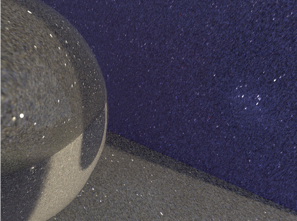
Although we weren’t able to perform realtime performance on reconstructed scenes, sample images are displayed below. At 1 sample per pixel, traversing the scene in realtime operated at around 1 frame per second.
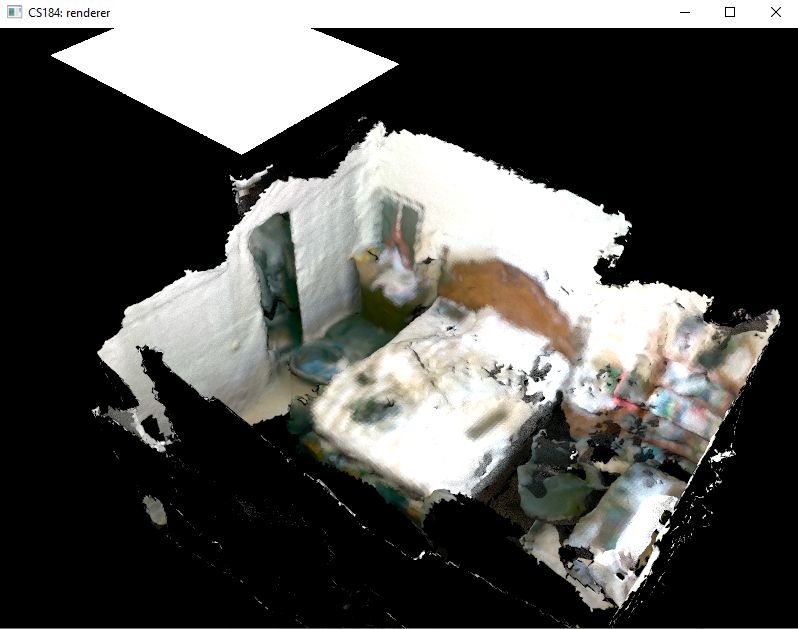
|
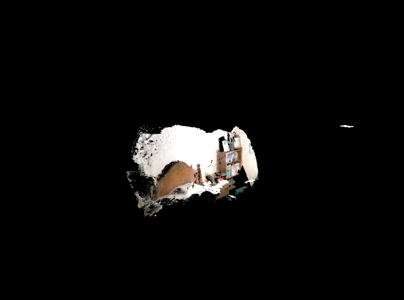
|
The GIF below demonstrates a traversal of a reconstructed scene with ray tracing. It is sped up by 10 times. Notice the noisy parts of the images, a result of only taking 1 sample per pixel.
|
|
References
- 3D Reconstruction (Open3D): [http://vladlen.info/papers/scene-reconstruction-POI.pdf]
- 3D Reconstruction (OpenARK): [https://www.youtube.com/watch?v=kDTkPS060T0]
Team Contributions
Adam was responsible for obtaining 3D reconstructions, processing the triangle meshes, and modifying the pathtracer pipeline to allow for large meshes with individually colored triangles.
Leo was responsible for the optimizations such as texture baking and bidirectional ray tracing to speed up the ray tracer to approach realtime performance.
Mitchell was responsible for using Blender to augment virtual scenes and helping process reconstructed real scenes to incorporate different BSDFs.